Visualise the distribution of a single continuous variable as a histogram
with a fading alpha gradient. Counts are drawn with rounded,
gradient-filled bars (like geom_col_fade() paired with
ggplot2::stat_bin()). Accepts all binning parameters forwarded to
ggplot2::stat_bin() (bins, binwidth, center, boundary, ...).
Usage
geom_histogram_fade(
  mapping = NULL,
  data = NULL,
  stat = "bin",
  position = "stack",
  ...,
  binwidth = NULL,
  bins = NULL,
  alpha_fade_to = 0,
  alpha_scope = "bar",
  orientation = NA,
  radius = grid::unit(0, "pt"),
  lineend = "butt",
  linejoin = "mitre",
  na.rm = FALSE,
  show.legend = NA,
  inherit.aes = TRUE
)
Arguments
- mapping
Set of aesthetic mappings created by
aes(). If specified andinherit.aes = TRUE(the default), it is combined with the default mapping at the top level of the plot. You must supplymappingif there is no plot mapping.- data
The data to be displayed in this layer. There are three options:
If
NULL, the default, the data is inherited from the plot data as specified in the call toggplot().A
data.frame, or other object, will override the plot data. All objects will be fortified to produce a data frame. Seefortify()for which variables will be created.A
functionwill be called with a single argument, the plot data. The return value must be adata.frame, and will be used as the layer data. Afunctioncan be created from aformula(e.g.~ head(.x, 10)).- stat
Use to override the default connection between
geom_histogram_fade()/geom_freqpoly_fade()andstat_bin().- position
A position adjustment to use on the data for this layer. This can be used in various ways, including to prevent overplotting and improving the display. The
positionargument accepts the following:The result of calling a position function, such as
position_jitter(). This method allows for passing extra arguments to the position.A string naming the position adjustment. To give the position as a string, strip the function name of the
position_prefix. For example, to useposition_jitter(), give the position as"jitter".For more information and other ways to specify the position, see the layer position documentation.
- ...
Other arguments passed on to
layer()'sparamsargument. These arguments broadly fall into one of 4 categories below. Notably, further arguments to thepositionargument, or aesthetics that are required can not be passed through.... Unknown arguments that are not part of the 4 categories below are ignored.Static aesthetics that are not mapped to a scale, but are at a fixed value and apply to the layer as a whole. For example,
colour = "red"orlinewidth = 3. The geom's documentation has an Aesthetics section that lists the available options. The 'required' aesthetics cannot be passed on to theparams. Please note that while passing unmapped aesthetics as vectors is technically possible, the order and required length is not guaranteed to be parallel to the input data.When constructing a layer using a
stat_*()function, the...argument can be used to pass on parameters to thegeompart of the layer. An example of this isstat_density(geom = "area", outline.type = "both"). The geom's documentation lists which parameters it can accept.Inversely, when constructing a layer using a
geom_*()function, the...argument can be used to pass on parameters to thestatpart of the layer. An example of this isgeom_area(stat = "density", adjust = 0.5). The stat's documentation lists which parameters it can accept.The
key_glyphargument oflayer()may also be passed on through.... This can be one of the functions described as key glyphs, to change the display of the layer in the legend.
- binwidth
Width of each bin in data units. When supplied, takes precedence over
bins. Forwarded toggplot2::stat_bin().- bins
Number of bins. Overridden by
binwidth. Defaults to 30. Forwarded toggplot2::stat_bin().- alpha_fade_to
A single finite number between 0 and 1. The alpha value at the baseline of each bar. Defaults to
0(fully transparent).- alpha_scope
How to choose the per-bar reference height that the gradient normalises against. The histogram family's vocabulary differs from
geom_col_fade()/geom_bar_fade()becausexis continuous (a binned variable) rather than a discrete category:"bar"(default),"group","fill","colour","global"– same meaning as ingeom_col_fade()."bin"– every bar in the same bin shares an alpha range. Useful underposition = "dodge"for highlighting the tallest group within each bin (e.g. "which species dominates each Sepal.Width bin").
The
"x"/"y"scopes accepted bygeom_col_fade()are not available here – on a continuous binned axis they would key onround(data$x), which buckets bins by integer rounding rather than by bin identity. Use"bin"for the per-bin meaning.- orientation
The orientation of the layer. The default (
NA) automatically determines the orientation from the aesthetic mapping. In the rare event that this fails it can be given explicitly by settingorientationto either"x"or"y". See the Orientation section for more detail.- radius
Corner radius passed to
grid::roundrectGrob(). Agrid::unit()object (e.g.unit(4, "pt")); a bare number is interpreted as points. Defaults tounit(0, "pt")(matchinggeom_bar()/geom_col()).- lineend
Line end style (round, butt, square).
- linejoin
Line join style (round, mitre, bevel).
- na.rm
If
FALSE, the default, missing values are removed with a warning. IfTRUE, missing values are silently removed.- show.legend
logical. Should this layer be included in the legends?
NA, the default, includes if any aesthetics are mapped.FALSEnever includes, andTRUEalways includes. It can also be a named logical vector to finely select the aesthetics to display. To include legend keys for all levels, even when no data exists, useTRUE. IfNA, all levels are shown in legend, but unobserved levels are omitted.- inherit.aes
If
FALSE, overrides the default aesthetics, rather than combining with them. This is most useful for helper functions that define both data and aesthetics and shouldn't inherit behaviour from the default plot specification, e.g.annotation_borders().
Value
A ggplot2::layer() object that can be added to a ggplot2::ggplot().
Aesthetics
geom_histogram_fade() understands the same aesthetics as
geom_col_fade() (it is GeomHistogramFade, a subclass of GeomColFade,
paired with ggplot2::stat_bin()). See ?geom_col_fade for the full
aesthetics table.
Orientation
This geom treats each axis differently and, thus, can thus have two orientations. Often the orientation is easy to deduce from a combination of the given mappings and the types of positional scales in use. Thus, ggplot2 will by default try to guess which orientation the layer should have. Under rare circumstances, the orientation is ambiguous and guessing may fail. In that case the orientation can be specified directly using the orientation parameter, which can be either "x" or "y". The value gives the axis that the geom should run along, "x" being the default orientation you would expect for the geom.
References
Murrell, P. (2022). "Vectorised Pattern Fills in R Graphics." Technical Report 2022-01, Department of Statistics, The University of Auckland. Version 1. https://www.stat.auckland.ac.nz/~paul/Reports/GraphicsEngine/vecpat/vecpat.html
See also
geom_col_fade() / geom_bar_fade() for the bar-chart equivalents,
geom_area_fade() for the general area-fade geom,
ggplot2::geom_histogram() and ggplot2::geom_freqpoly() for the
non-fading originals.
Examples
library(ggplot2)
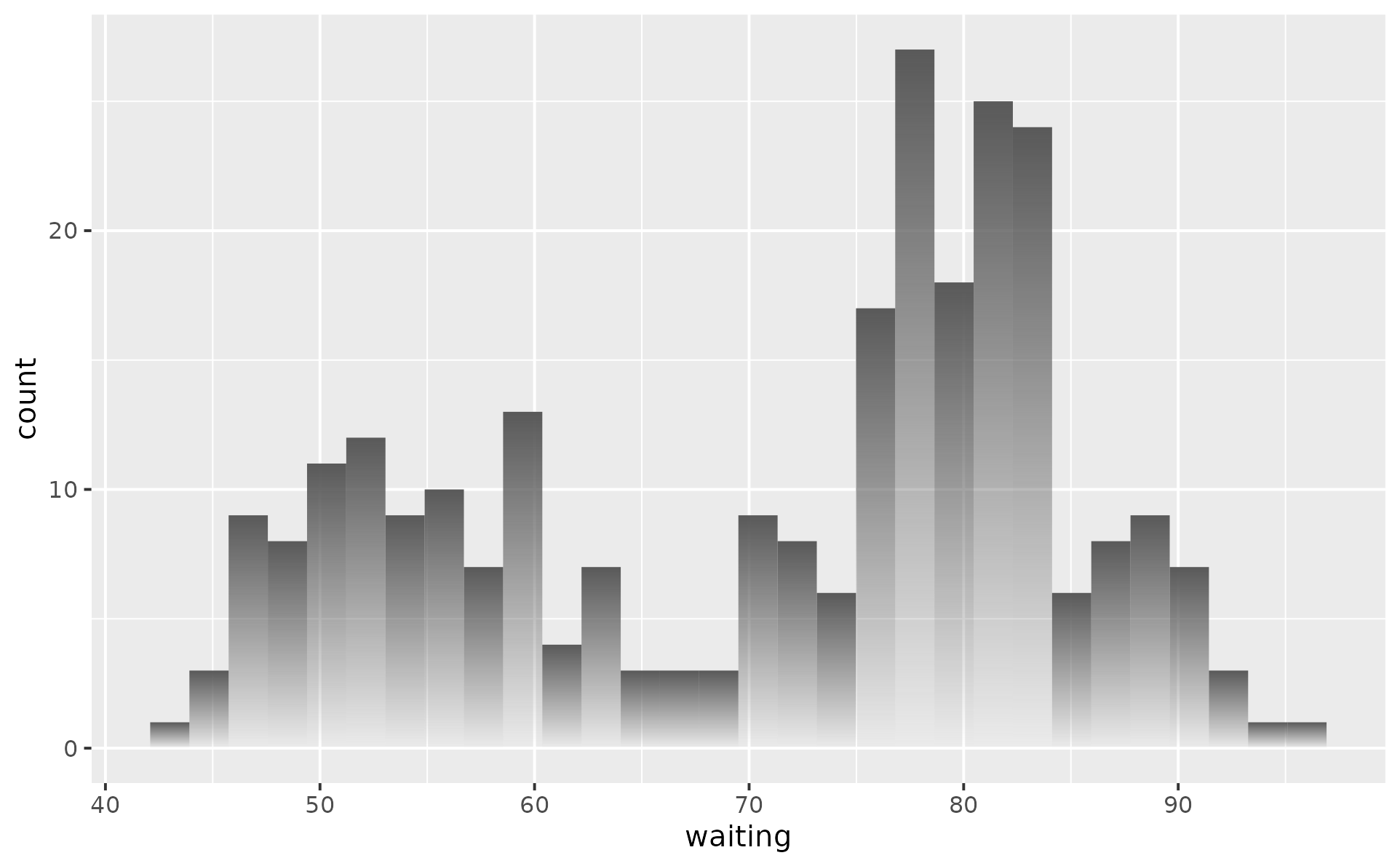
# By default each bar has its own alpha scope
p <- ggplot(faithful, aes(waiting))
p + geom_histogram_fade()
#> `stat_bin()` using `bins = 30`. Pick better value `binwidth`.
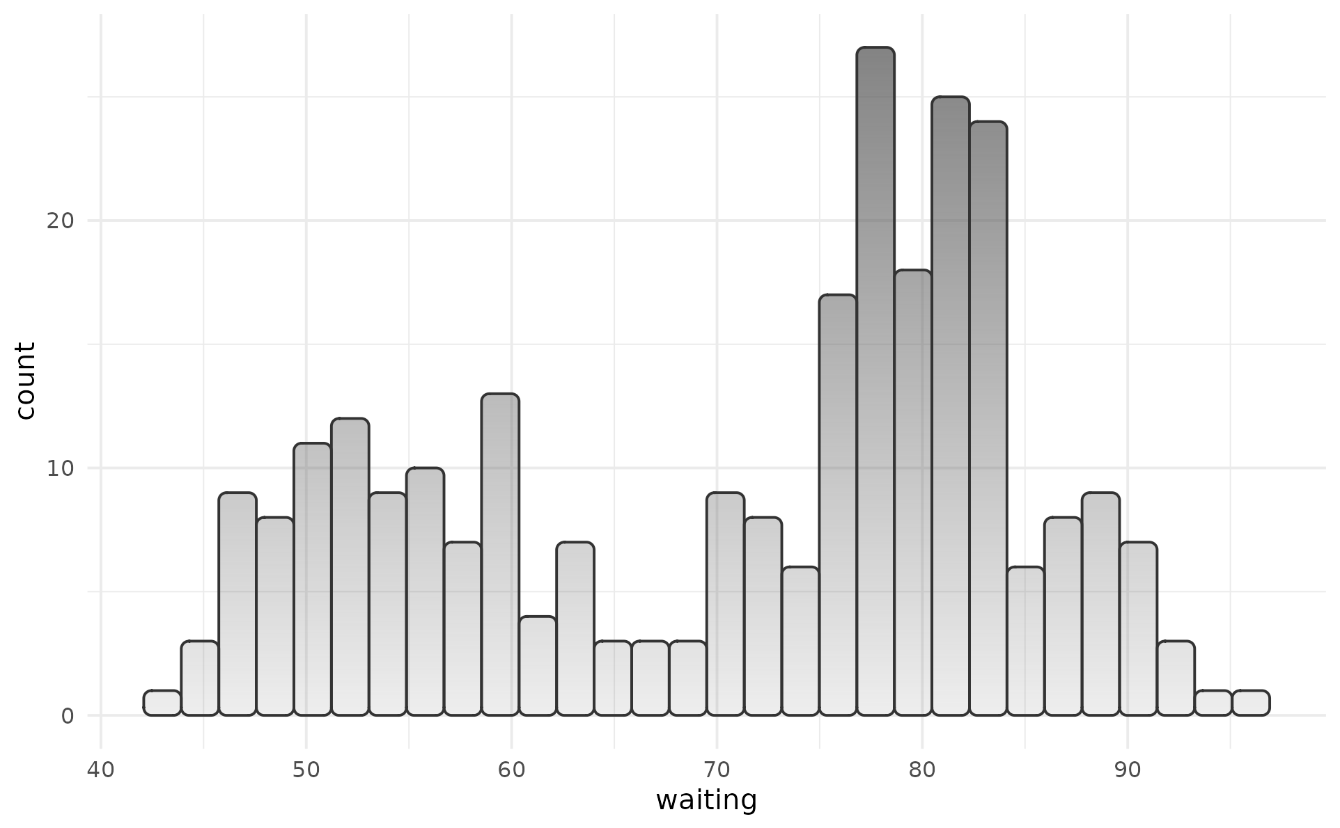
 # when all bars shall share the same alpha scope,
# set alpha_scope = "global"
p +
geom_histogram_fade(
alpha_scope = "global",
alpha = 0.75,
alpha_fade_to = 0.1,
radius = unit(3, "pt"),
colour = "#333333"
) +
theme_minimal()
#> `stat_bin()` using `bins = 30`. Pick better value `binwidth`.
# when all bars shall share the same alpha scope,
# set alpha_scope = "global"
p +
geom_histogram_fade(
alpha_scope = "global",
alpha = 0.75,
alpha_fade_to = 0.1,
radius = unit(3, "pt"),
colour = "#333333"
) +
theme_minimal()
#> `stat_bin()` using `bins = 30`. Pick better value `binwidth`.
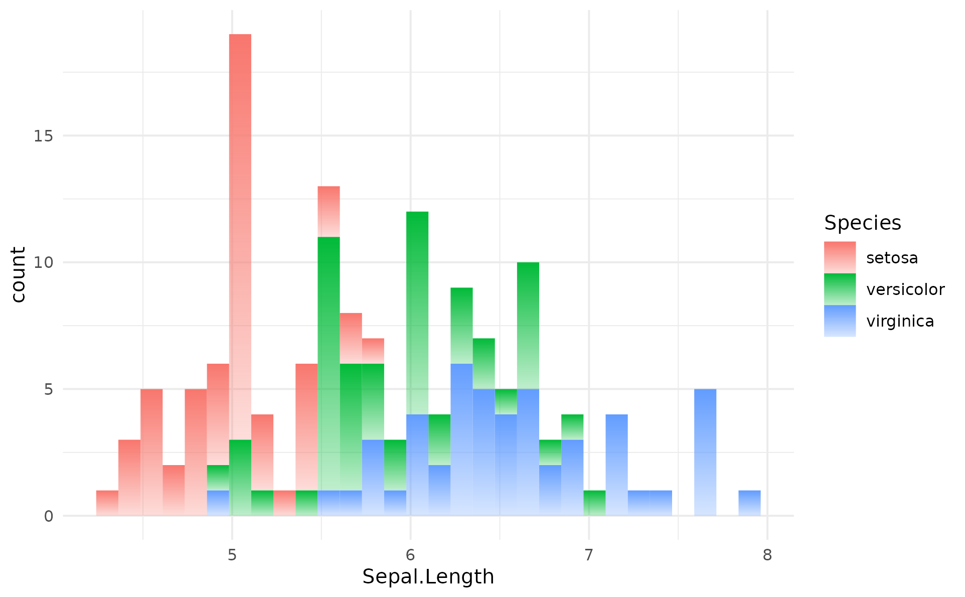
 # Stacked histogram with groups
ggplot(iris, aes(Sepal.Length, fill = Species)) +
geom_histogram_fade(alpha_fade_to = 0.25) +
theme_minimal()
#> `stat_bin()` using `bins = 30`. Pick better value `binwidth`.
# Stacked histogram with groups
ggplot(iris, aes(Sepal.Length, fill = Species)) +
geom_histogram_fade(alpha_fade_to = 0.25) +
theme_minimal()
#> `stat_bin()` using `bins = 30`. Pick better value `binwidth`.
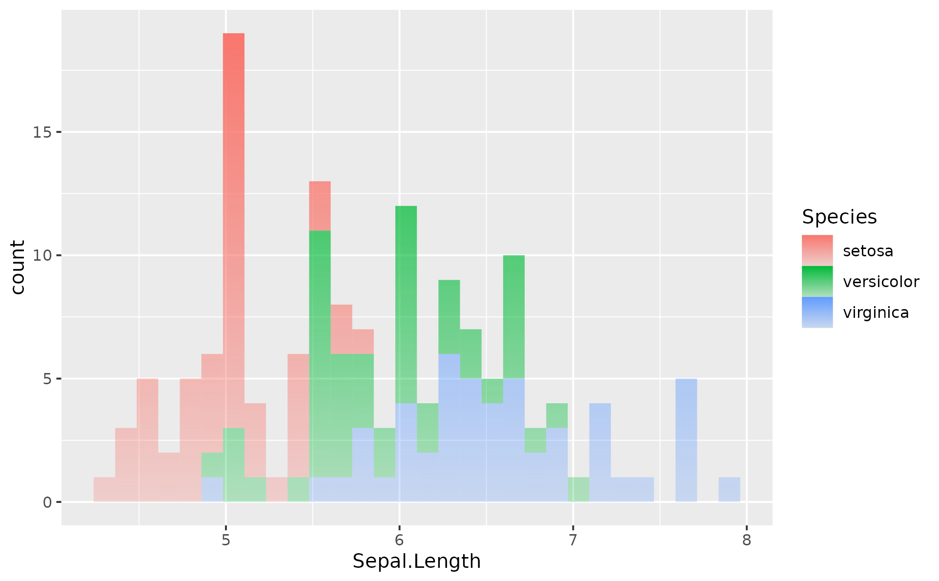
 # Stacked histogram with groups and global alpha scope
ggplot(iris, aes(Sepal.Length, fill = Species)) +
geom_histogram_fade(
alpha_fade_to = 0.25,
alpha_scope = "global"
)
#> `stat_bin()` using `bins = 30`. Pick better value `binwidth`.
# Stacked histogram with groups and global alpha scope
ggplot(iris, aes(Sepal.Length, fill = Species)) +
geom_histogram_fade(
alpha_fade_to = 0.25,
alpha_scope = "global"
)
#> `stat_bin()` using `bins = 30`. Pick better value `binwidth`.
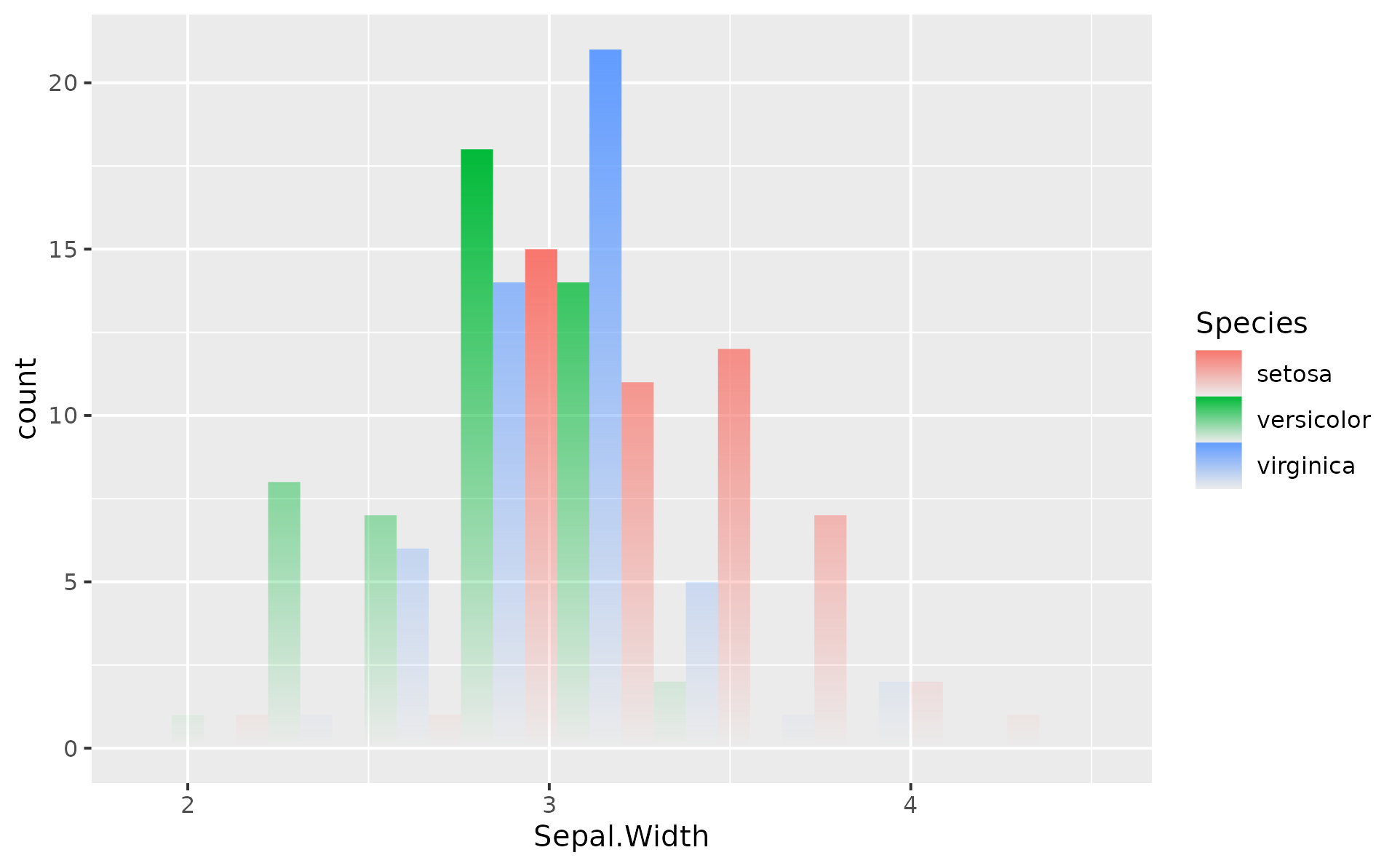
 # Per-fill scope under position = "dodge": each fill cluster has its own
# alpha range, so the tallest sub-bar in every bin reaches full opacity.
ggplot(iris, aes(Sepal.Width, fill = Species)) +
geom_histogram_fade(
position = "dodge",
bins = 10,
alpha_scope = "fill"
)
# Per-fill scope under position = "dodge": each fill cluster has its own
# alpha range, so the tallest sub-bar in every bin reaches full opacity.
ggplot(iris, aes(Sepal.Width, fill = Species)) +
geom_histogram_fade(
position = "dodge",
bins = 10,
alpha_scope = "fill"
)