Line Segments with a Fading Gradient
Source:R/geom-segment-fade.R, R/geom-curve-fade.R
geom_segment_fade.Rdgeom_segment_fade() draws line segments like ggplot2::geom_segment()
but applies an alpha gradient along each segment so that one or both ends
fade to transparent. The gradient direction follows the segment (from
(x, y) to (xend, yend)), so it works at any angle.
Rendering requires a graphics device that supports clipping paths
(e.g. ragg, cairo, svg).
Usage
geom_segment_fade(
  mapping = NULL,
  data = NULL,
  stat = "identity",
  position = "identity",
  ...,
  alpha_fade_to = 0,
  fade_direction = "start",
  arrow = NULL,
  arrow.fill = NULL,
  lineend = "butt",
  linejoin = "round",
  na.rm = FALSE,
  show.legend = NA,
  inherit.aes = TRUE
)

geom_curve_fade(
  mapping = NULL,
  data = NULL,
  stat = "identity",
  position = "identity",
  ...,
  alpha_fade_to = 0,
  fade_direction = "start",
  curve_count_cap = 200,
  curvature = 0.5,
  angle = 90,
  ncp = 5,
  arrow = NULL,
  arrow.fill = NULL,
  lineend = "butt",
  na.rm = FALSE,
  show.legend = NA,
  inherit.aes = TRUE
)
Arguments
- mapping
Set of aesthetic mappings created by
aes(). If specified andinherit.aes = TRUE(the default), it is combined with the default mapping at the top level of the plot. You must supplymappingif there is no plot mapping.- data
The data to be displayed in this layer. There are three options:
If
NULL, the default, the data is inherited from the plot data as specified in the call toggplot().A
data.frame, or other object, will override the plot data. All objects will be fortified to produce a data frame. Seefortify()for which variables will be created.A
functionwill be called with a single argument, the plot data. The return value must be adata.frame, and will be used as the layer data. Afunctioncan be created from aformula(e.g.~ head(.x, 10)).- stat
The statistical transformation to use on the data for this layer. When using a
geom_*()function to construct a layer, thestatargument can be used to override the default coupling between geoms and stats. Thestatargument accepts the following:A
Statggproto subclass, for exampleStatCount.A string naming the stat. To give the stat as a string, strip the function name of the
stat_prefix. For example, to usestat_count(), give the stat as"count".For more information and other ways to specify the stat, see the layer stat documentation.
- position
A position adjustment to use on the data for this layer. This can be used in various ways, including to prevent overplotting and improving the display. The
positionargument accepts the following:The result of calling a position function, such as
position_jitter(). This method allows for passing extra arguments to the position.A string naming the position adjustment. To give the position as a string, strip the function name of the
position_prefix. For example, to useposition_jitter(), give the position as"jitter".For more information and other ways to specify the position, see the layer position documentation.
- ...
Other arguments passed on to
layer()'sparamsargument. These arguments broadly fall into one of 4 categories below. Notably, further arguments to thepositionargument, or aesthetics that are required can not be passed through.... Unknown arguments that are not part of the 4 categories below are ignored.Static aesthetics that are not mapped to a scale, but are at a fixed value and apply to the layer as a whole. For example,
colour = "red"orlinewidth = 3. The geom's documentation has an Aesthetics section that lists the available options. The 'required' aesthetics cannot be passed on to theparams. Please note that while passing unmapped aesthetics as vectors is technically possible, the order and required length is not guaranteed to be parallel to the input data.When constructing a layer using a
stat_*()function, the...argument can be used to pass on parameters to thegeompart of the layer. An example of this isstat_density(geom = "area", outline.type = "both"). The geom's documentation lists which parameters it can accept.Inversely, when constructing a layer using a
geom_*()function, the...argument can be used to pass on parameters to thestatpart of the layer. An example of this isgeom_area(stat = "density", adjust = 0.5). The stat's documentation lists which parameters it can accept.The
key_glyphargument oflayer()may also be passed on through.... This can be one of the functions described as key glyphs, to change the display of the layer in the legend.
- alpha_fade_to
A single finite number between 0 and 1. The alpha value at the fading end(s). Defaults to
0(fully transparent).- fade_direction
Which end(s) of each segment fade? A character vector containing
"start"(the(x, y)end fades),"end"(the(xend, yend)end fades), or bothc("start", "end"). Defaults to"start".- arrow
specification for arrow heads, as created by
grid::arrow().- arrow.fill
fill colour to use for the arrow head (if closed).
NULLmeans usecolouraesthetic.- lineend
Line end style (round, butt, square).
- linejoin
Line join style (round, mitre, bevel).
- na.rm
If
FALSE, the default, missing values are removed with a warning. IfTRUE, missing values are silently removed.- show.legend
logical. Should this layer be included in the legends?
NA, the default, includes if any aesthetics are mapped.FALSEnever includes, andTRUEalways includes. It can also be a named logical vector to finely select the aesthetics to display. To include legend keys for all levels, even when no data exists, useTRUE. IfNA, all levels are shown in legend, but unobserved levels are omitted.- inherit.aes
If
FALSE, overrides the default aesthetics, rather than combining with them. This is most useful for helper functions that define both data and aesthetics and shouldn't inherit behaviour from the default plot specification, e.g.annotation_borders().- curve_count_cap
Soft cap on the number of curves
geom_curve_fade()will composite per panel. OnegroupGrob(op = "dest.in")is built per curve, so render cost scales roughly linearly at ~30 ms / curve. Past the cap the layer falls back to plainggplot2::geom_curve()(no fade) and emits a warning. Default200(~6 s worst case). PassInfto disable. For bulk fading, usegeom_path_fade()orgeom_segment_fade()instead.- curvature
A numeric value giving the amount of curvature. Negative values produce left-hand curves, positive values produce right-hand curves, and zero produces a straight line.
- angle
A numeric value between 0 and 180, giving an amount to skew the control points of the curve. Values less than 90 skew the curve towards the start point and values greater than 90 skew the curve towards the end point.
- ncp
The number of control points used to draw the curve. More control points creates a smoother curve.
Value
A ggplot2::layer() object that can be added to a ggplot2::ggplot().
Details
Non-linear coordinate systems
Under non-linear coordinates such as ggplot2::coord_polar() and
ggplot2::coord_radial() the user-supplied endpoints (x, y) and
(xend, yend) are transformed to device space and connected by a
straight chord – exactly as ggplot2::geom_segment() does. The fade is
then applied along that chord, so both endpoint positions and the fade
direction are consistent with the unfaded geom.
If you want the line to follow a curve implied by the coord system
(for example a circle at constant y under polar), use
geom_hline_fade() / geom_vline_fade() / geom_abline_fade() instead –
those geoms subdivide the line in data space so the fade tracks the
curve, not a chord.
Self-crossing paths
When a faded path crosses itself, the pixels at the crossing are rasterised once per overlapping segment, and the per-segment alpha values compound. Where the two strands carry different alphas (one near the faded end, one near the opaque end), the crossing appears noticeably darker than either strand alone.
This behaviour is inherent to how semi-transparent strokes are
alpha-blended at the device level, not specific to geom_path_fade() –
the same effect appears with ggplot2::geom_path(alpha = 0.5). There is
no general workaround at the rendering layer; if a clean intersection
matters for your plot, the practical options are:
Raise
alpha_fade_toso the strands at both ends are closer in opacity (smaller delta -> less visible darkening).Use a fully opaque stroke (no fade) for paths known to self-cross.
Restructure the data so the crossing is split across separate layers.
Applies equally to geom_segment_fade() and geom_curve_fade() when
two segments / curves overlap at the same pixel.
References
Murrell, P., Pedersen, T. L., and Skintzos, P. (2023). "Porter-Duff Compositing Operators in R Graphics." Department of Statistics, The University of Auckland. Version 1. https://www.stat.auckland.ac.nz/~paul/Reports/GraphicsEngine/compositing/compositing.html
Murrell, P. (2023). "Groups, Compositing Operators, and Affine Transformations in R Graphics." Technical Report 2021-02, Department of Statistics, The University of Auckland. Version 3. https://www.stat.auckland.ac.nz/~paul/Reports/GraphicsEngine/groups/groups.html
See also
geom_path_fade() for connected paths with alpha fading,
ggplot2::geom_segment() and ggplot2::geom_curve()
for the unfaded versions.
Aesthetics
geom_segment_fade() understands the following aesthetics. Required aesthetics are displayed in bold and defaults are displayed for optional aesthetics:
| • | x | |
| • | y | |
| • | xend | |
| • | yend | |
| • | alpha | → NA |
| • | colour | → via theme() |
| • | group | → inferred |
| • | linetype | → via theme() |
| • | linewidth | → via theme() |
Learn more about setting these aesthetics in vignette("ggplot2-specs").
Examples
library(ggplot2)
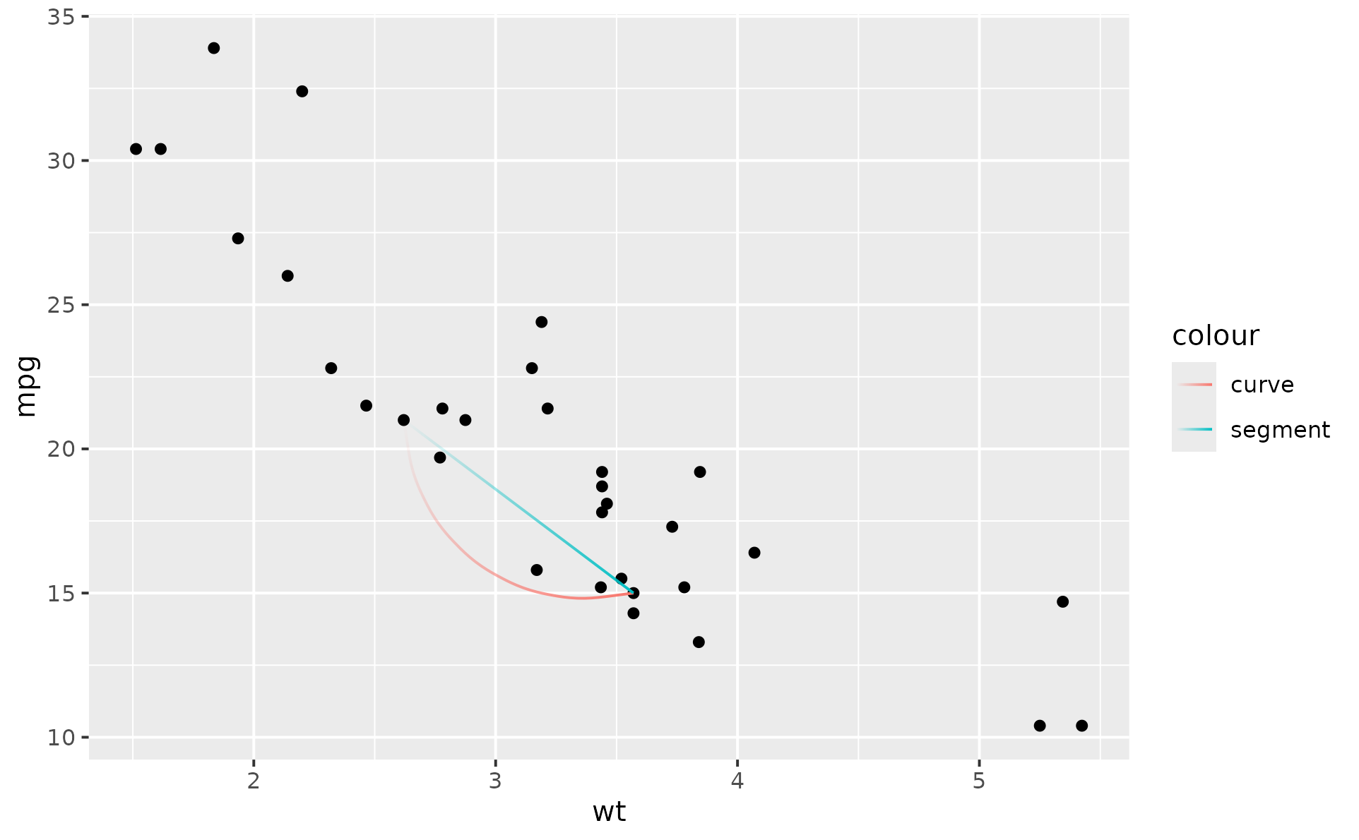
b <- ggplot(mtcars, aes(wt, mpg)) +
geom_point()
df <- data.frame(x1 = 2.62, x2 = 3.57, y1 = 21.0, y2 = 15.0)
b +
geom_curve_fade(
aes(x = x1, y = y1, xend = x2, yend = y2, colour = "curve"),
data = df
) +
geom_segment_fade(
aes(x = x1, y = y1, xend = x2, yend = y2, colour = "segment"),
data = df
)
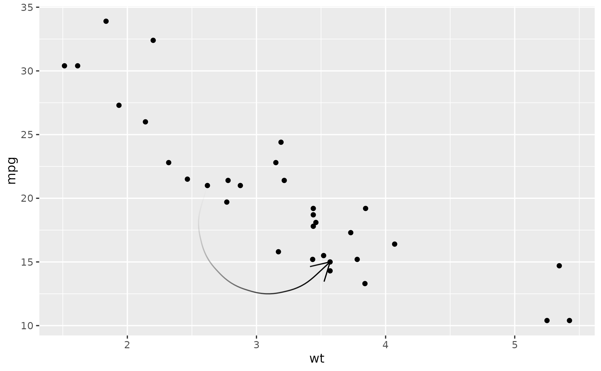
 b +
geom_curve_fade(
aes(x = x1, y = y1, xend = x2, yend = y2),
data = df,
curvature = 1,
fade_direction = "start",
arrow = grid::arrow()
)
b +
geom_curve_fade(
aes(x = x1, y = y1, xend = x2, yend = y2),
data = df,
curvature = 1,
fade_direction = "start",
arrow = grid::arrow()
)
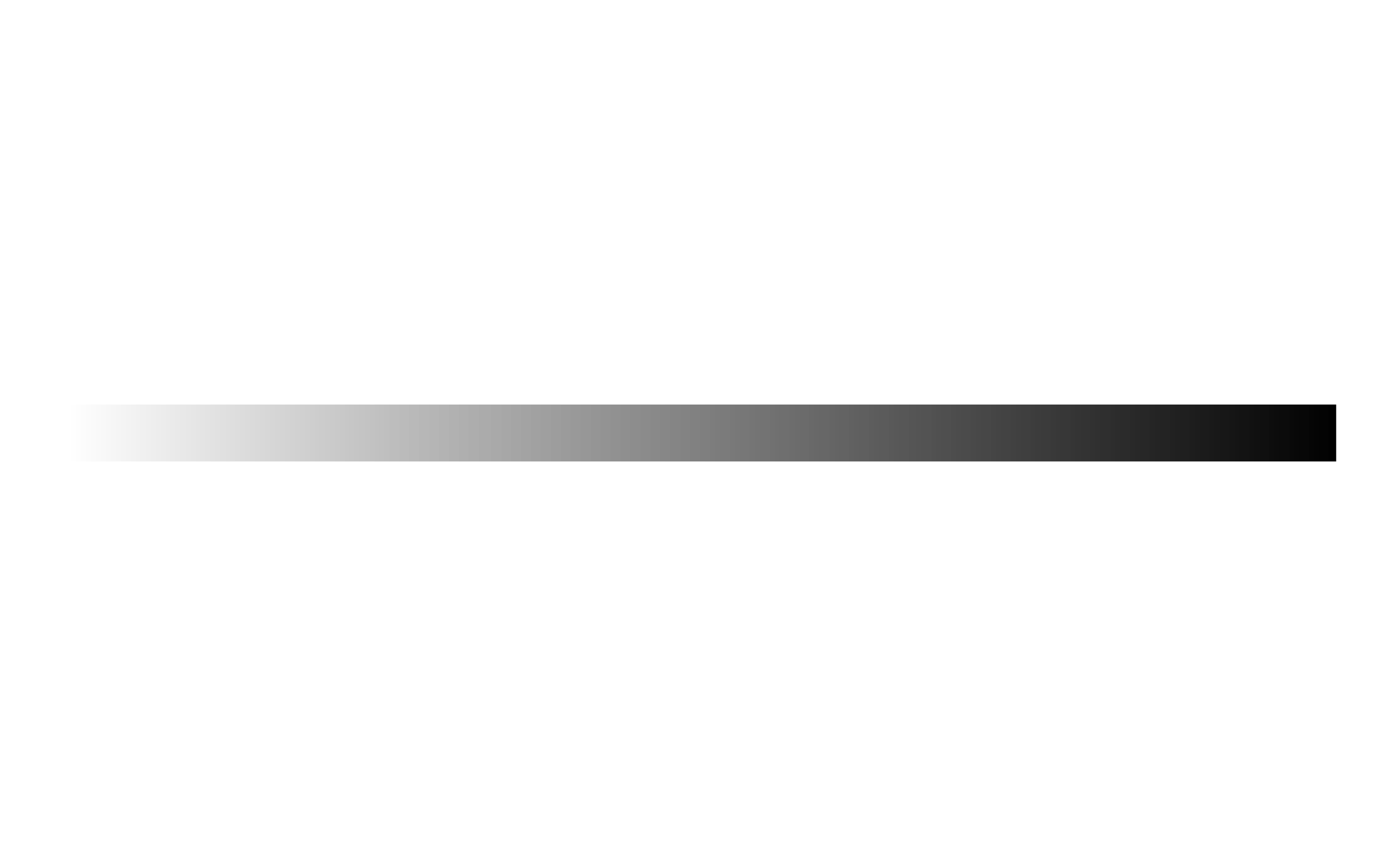
 df <- data.frame(x1 = 1, x2 = 9, y1 = 1, y2 = 1)
p <- ggplot(df, aes(x)) +
theme_void()
# Basic example with default fade_direction
p +
geom_segment_fade(
aes(x = x1, y = y1, xend = x2, yend = y2),
fade_direction = "start", # default
linewidth = 10
)
df <- data.frame(x1 = 1, x2 = 9, y1 = 1, y2 = 1)
p <- ggplot(df, aes(x)) +
theme_void()
# Basic example with default fade_direction
p +
geom_segment_fade(
aes(x = x1, y = y1, xend = x2, yend = y2),
fade_direction = "start", # default
linewidth = 10
)
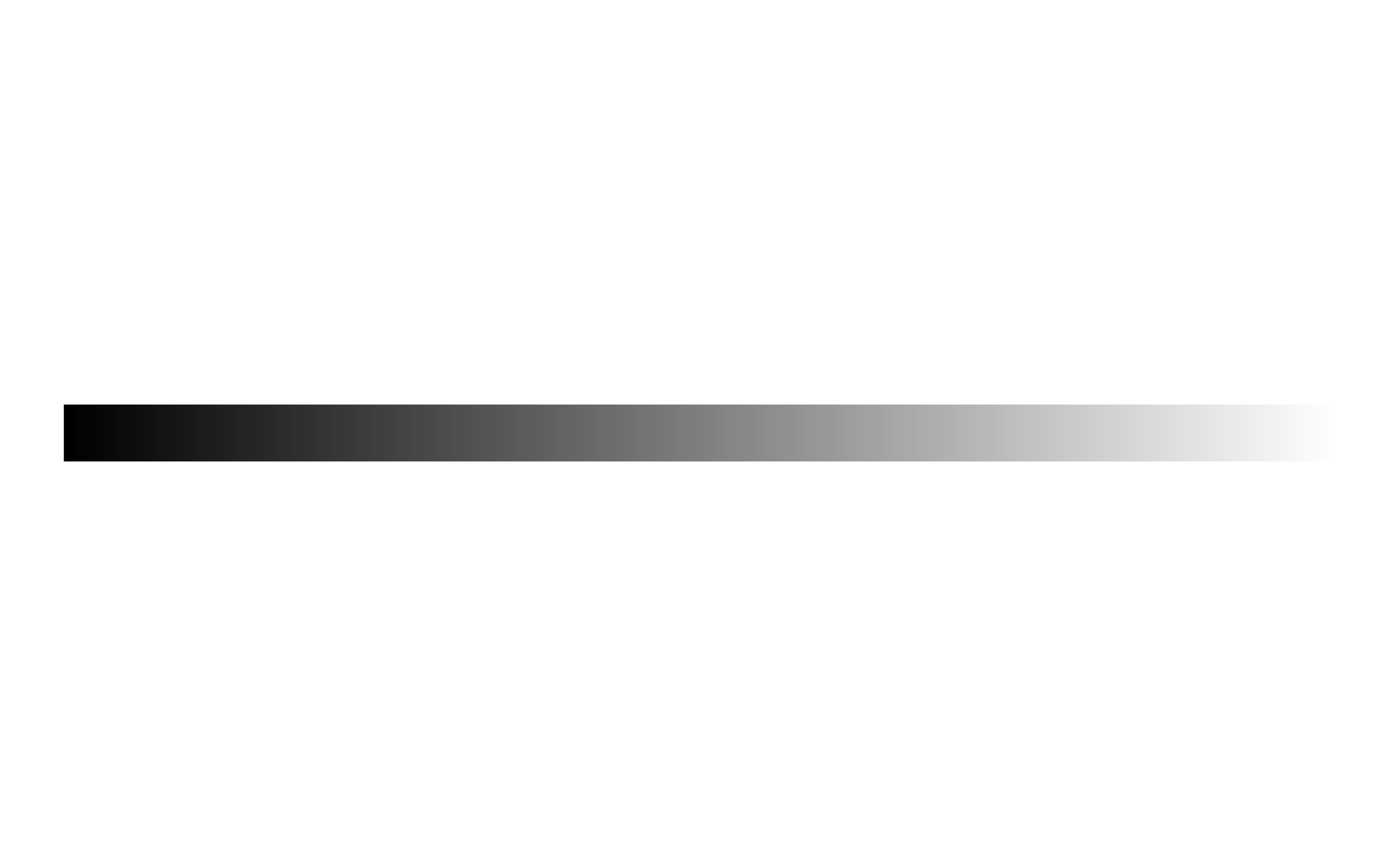
 # Change fade_direction towards start
p +
geom_segment_fade(
aes(x = x1, y = y1, xend = x2, yend = y2),
fade_direction = "end",
linewidth = 10
)
# Change fade_direction towards start
p +
geom_segment_fade(
aes(x = x1, y = y1, xend = x2, yend = y2),
fade_direction = "end",
linewidth = 10
)
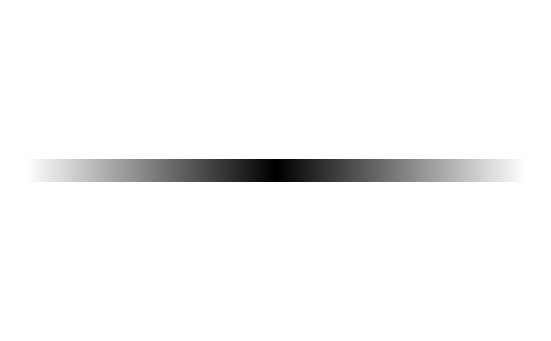
 # Fade from centre to both sides
p +
geom_segment_fade(
aes(x = x1, y = y1, xend = x2, yend = y2),
fade_direction = c("start", "end"),
linewidth = 10
)
# Fade from centre to both sides
p +
geom_segment_fade(
aes(x = x1, y = y1, xend = x2, yend = y2),
fade_direction = c("start", "end"),
linewidth = 10
)