BDEW Standard Load Profiles for Electricity and Gas • standardlastprofile

Standard load profiles (SLPs) for electricity and gas, published by the German Association of Energy and Water Industries (BDEW Bundesverband der Energie- und Wasserwirtschaft e.V.). SLPs are used by utilities, distribution network operators, and the energy industry to forecast demand for customer groups that are not continuously metered.

Small multiple line chart of 11 electricity standard load profiles
from 1999 published by the German Association of Energy and Water Industries
(BDEW). Lines compare three seasonal periods across different day types.

Installation

install.packages("standardlastprofile")

Included features

slp_info() — descriptions for all electricity and gas profile IDs

Electricity

slp_electricity() — generate a 15-minute profile for any date range
slp_electricity_profiles — dataset of BDEW electricity SLPs in tidy format

Gas

slp_gas() — generate daily gas consumption via the SigLinDe method
slp_gas_coefficients() — retrieve SigLinDe coefficients for gas SLPs
slp_gas_kundenwert() — derive the customer value (German: “Kundenwert”) from a reference temperature series
slp_gas_siglinde() — low-level SigLinDe function, can be useful for custom or region-specific SigLinDe coefficients
slp_gas_weekday_factors() — retrieve weekday factors for gas SLPs

Electricity

The dataset slp_electricity_profiles contains 26,784 observations across 5 variables:

profile_id: load profile identifier
period: "summer", "winter", or "transition" for 1999 profiles; a lowercase month name for 2025 profiles
day: "workday", "saturday", or "sunday"
timestamp: quarter-hour start time in "%H:%M" format
watts: average electric power, normalised to 1,000 kWh/a

str(slp_electricity_profiles)
#> 'data.frame':    26784 obs. of  5 variables:
#>  $ profile_id: chr  "H0" "H0" "H0" "H0" ...
#>  $ period    : chr  "winter" "winter" "winter" "winter" ...
#>  $ day       : chr  "saturday" "saturday" "saturday" "saturday" ...
#>  $ timestamp : chr  "00:00" "00:15" "00:30" "00:45" ...
#>  $ watts     : num  70.8 68.2 65.9 63.3 59.5 55 50.5 46.6 43.9 42.3 ...

1999 profiles

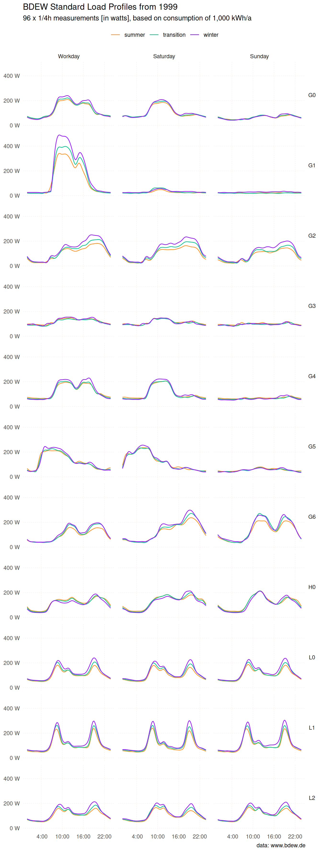
Based on an analysis of 1,209 load profiles of low-voltage electricity consumers in Germany¹:

H0: households
G0–G6: commercial
L0–L2: agriculture

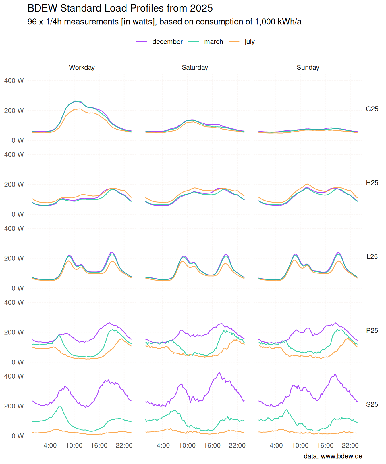
2025 profiles

An updated set published by BDEW in 2025, reflecting changes in consumption patterns since the original study. Unlike the 1999 profiles (three seasonal periods), the 2025 profiles provide values for each calendar month:

H25, G25, L25: updated household, commercial, and agriculture profiles
P25: households with a photovoltaic (PV) system
S25: households with a PV system and battery storage

Small multiple line chart of five electricity standard load profiles
published by BDEW in 2025. Lines are coloured by calendar month and faceted
by profile and day type.

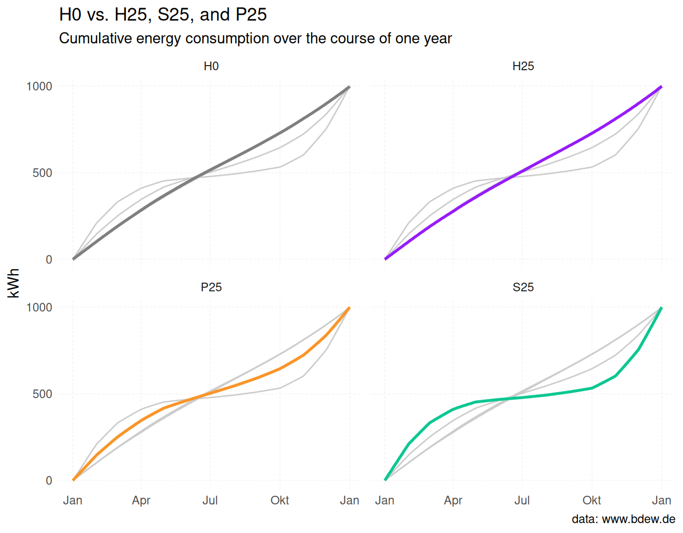
The chart below compares cumulative energy consumption of the 2025 household profiles against H0 over a full year. H25 tracks H0 closely; P25 and S25 flatten from spring through summer as solar generation and storage reduce grid draw.

Faceted line plot with four panels for H0, H25, P25, and S25.
Each panel shows cumulative energy consumption in kWh over 2026.
A grey reference line shows H0. H25 tracks H0 closely, while P25 and S25
diverge from spring onwards due to photovoltaic generation and battery storage.

Generate a profile

slp_electricity() returns a data frame with one row per 15-minute interval:

G5 <- slp_electricity(
  profile_id = "G5",
  start_date = "2023-12-22",
  end_date   = "2023-12-27"
)

head(G5)
#>   profile_id          start_time            end_time watts
#> 1         G5 2023-12-22 00:00:00 2023-12-22 00:15:00  50.1
#> 2         G5 2023-12-22 00:15:00 2023-12-22 00:30:00  47.4
#> 3         G5 2023-12-22 00:30:00 2023-12-22 00:45:00  44.9
#> 4         G5 2023-12-22 00:45:00 2023-12-22 01:00:00  43.3
#> 5         G5 2023-12-22 01:00:00 2023-12-22 01:15:00  43.0
#> 6         G5 2023-12-22 01:15:00 2023-12-22 01:30:00  43.8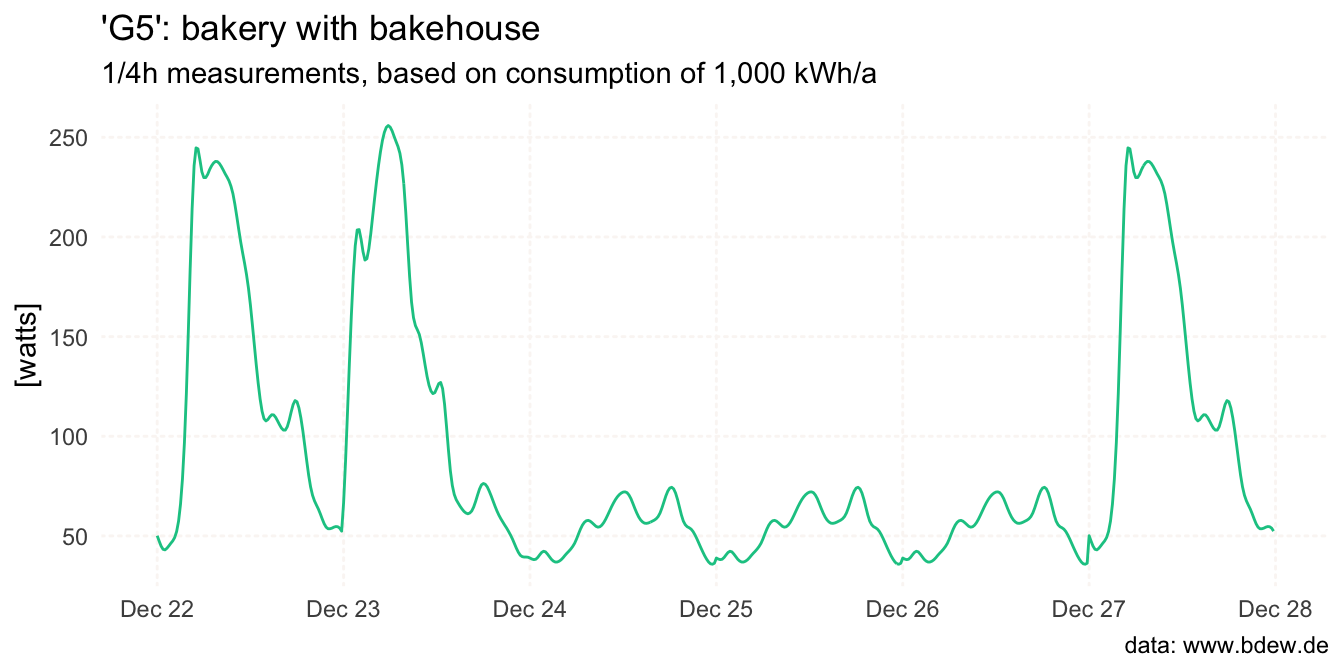

Line plot of the electricity standard load profile 'G5' (bakery
with a bakehouse) from December 22nd to 27th 2023, normalised to 1,000 kWh/a.

Public holidays

Both slp_electricity() and slp_gas() use the same holiday logic: nine nationwide German public holidays are treated as Sundays by default:

New Year’s
Good Friday
Easter Monday
Labour Day
Ascension Day
Whit Monday
German Unity Day
Christmas Day
Boxing Day

State-level holidays are not included because they vary by state and year. Use the holidays argument in either function to supply your own dates — the built-in data are then ignored entirely. See the electricity article for an example of how to fetch state-level holidays from the nager.Date API.

Gas

slp_gas() implements the BDEW/VKU/GEODE synthetic procedure (SigLinDe method) for daily gas consumption. The gas consumption on any particular day is influenced by three factors:

outside temperature
personal preferences (kundenwert)
the day of the week

slp_gas() hence takes a date vector for which the gas consumption should be calculated, a vector of daily mean temperatures and a kundenwert (customer value in kWh/day), together with one of 15 gas profile IDs.

Pass dates and temps to slp_gas() together with the kundenwert.

The kundenwert of 55.1 kWh/day is itself derived once, from the customer’s annual consumption and a reference temperature series. See the gas article for that step and the full method.

The result of slp_gas() is a data frame with three columns: profile_id, date, and kwh which is the daily gas consumption:

HEF <- slp_gas("HEF", dates, temps, kundenwert = 55.1)
head(HEF)
#>   profile_id       date      kwh
#> 1        HEF 2025-10-01 40.95047
#> 2        HEF 2025-10-02 32.50304
#> 3        HEF 2025-10-03 31.91795
#> 4        HEF 2025-10-04 27.32729
#> 5        HEF 2025-10-05 32.50304
#> 6        HEF 2025-10-06 30.17767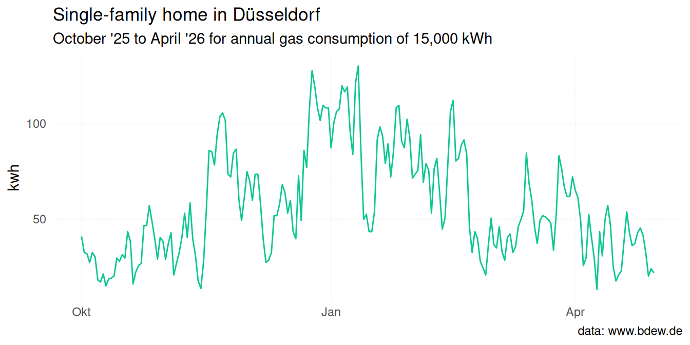

Line chart of daily gas consumption in kilowatt-hours for a
single-family home in Düsseldorf across the 2025/26 heating season. Demand
peaks in the cold winter months and is lowest in the mild shoulder months of
October and April.

In the example above we assumed a single-family home (profile HEF) in Düsseldorf.

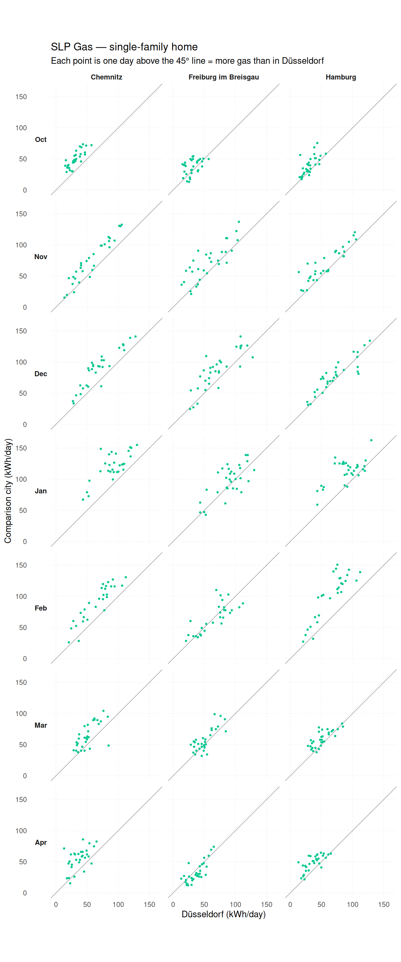
In the following graph, we compare the same customer (i.e. we set the kundenwert) for the same period – October 2025 to April 2026 – with three other locations. This allows us to isolate the influence of the outside temperature on gas consumption in these cities:

Chemnitz,
Freiburg im Breisgau, and
Hamburg.

Each point represents a single day in the period from 1 October 2025 to 30 April 2026. Points above the 45° line indicate that the customer would have consumed more gas than in Düsseldorf. We can see that this winter was colder in all three cities than in Düsseldorf, so all the points lie above the line – most notably in Chemnitz, least so in Freiburg im Breisgau, with Hamburg in between:

Faceted scatterplot grid: columns are Chemnitz, Freiburg im Breisgau, Hamburg;
rows are months October to April. Each point is a day; the x-axis is daily
gas consumption in Düsseldorf, the y-axis in the comparison city, with a
45-degree reference line. All three cities' point clouds sit above the line
in winter, most clearly for Chemnitz.

For a detailed explanation of the SigLinDe parameters and the full climate zone comparison, see the gas articles on the package website.

Sources

Electricity SLPs: https://www.bdew.de/energie/standardlastprofile-strom/
Gas SLPs: https://www.bdew.de/energie/standardlastprofile-gas/

Code of Conduct

Please note that this project is released with a Contributor Code of Conduct. By participating in this project you agree to abide by its terms.