Generate a standard load profile

Standard load profiles are crucial for electricity providers, grid operators, and the energy industry as a whole. They aid in planning and optimizing the demand for electricity generation and distribution. Additionally, they serve as the foundation for billing and balancing electricity quantities in the energy market. For smaller consumers, the financial expense of continuous consumption measurement is often unreasonable. Energy supply companies can therefore use a standard load profile as the basis for creating a consumption forecast.

The aim of this vignette is to show how the algorithm of the slp_generate() function works.¹ The data in the slp dataset forms the basis for all subsequent steps.

head(slp)
#>   profile_id period      day timestamp watts
#> 1         H0 winter saturday     00:00  70.8
#> 2         H0 winter saturday     00:15  68.2
#> 3         H0 winter saturday     00:30  65.9
#> 4         H0 winter saturday     00:45  63.3
#> 5         H0 winter saturday     01:00  59.5
#> 6         H0 winter saturday     01:15  55.0

There are 96 x 1/4 hour measurements of electrical power for each unique combination of profile_id, period and day, which we refer to as the “standard load profile”. The value for “00:00” indicates the average work done in the morning between 00:00 and 00:15. The data was collected and analyzed in 1999 and is provided by German Association of Energy and Water Industries (BDEW Bundesverband der Energie- und Wasserwirtschaft e.V.).²

Those measurements are normalized to an annual consumption of 1,000 kWh. So, if we sum up all the quarter-hour consumption values for a year, the result is (approximately) 1,000 kWh/year.

library(standardlastprofile)
H0_2024 <- slp_generate(
  profile_id = "H0",
  start_date = "2024-01-01",
  end_date = "2024-12-31"
  )

sum(H0_2024$watts)
#> [1] 4008335

‘Hold on - didn’t you just say 1,000?!’, you might be thinking. Yes, you are correct; we must convert power units into energy units. The values returned are 1/4-hour measurements in watts. To convert the values to watt-hours, we must, therefore, divide them by 4. Since one watt-hour is equal to 1/1000 kilowatt-hour, we also divide by 1,000:

sum(H0_2024$watts / 4 / 1000)
#> [1] 1002.084

Algorithm step by step

When you call slp_generate(), you generate (surprise!) a standard load profile. These are the steps that are then performed:

1. Generate a date sequence from start_date to end_date.

2. Map each day to combination of day and period.

3. Use result from 2nd step to extract values from slp.³

4. Apply polynomial function to values of profile identifier H0.

5. Return data.

Generate a date sequence

In the initial step, a date sequence is created from start_date to end_date based on the user input. Here’s a simple example:

start <- as.Date("2023-12-22")
end <- as.Date("2023-12-27")

(date_seq <- seq.Date(start, end, by = "day"))
#> [1] "2023-12-22" "2023-12-23" "2023-12-24" "2023-12-25" "2023-12-26"
#> [6] "2023-12-27"

Map each day to a period and a weekday

The measured load profiles analyzed in the study showed that electricity consumption across all groups fluctuates both over the period of a year and over the days within a week. The period definition is:

• summer: May 15 to September 14
• winter: November 1 to March 20
• transition: March 21 to May 14, and September 15 to October 31

It was also found that there was no significant difference in consumption on weekdays from Monday to Friday for any group. For this reason, the days Monday to Friday are grouped together as ‘workdays’. December 24th and 31st are considered Saturdays too if they are not Sundays. Public holidays are regarded as Sundays.

Note: The package standardlastprofile supports only public holidays for Germany. Those were retrieved from the nager.Date API. Below are nationwide holidays for 2024:

• Jan 1: New Year’s
• Mar 29: Good Friday
• Apr 1: Easter Monday
• May 1: Labor Day
• May 9: Ascension Day
• May 20: Whit Monday
• Oct 3: German Unity Day
• Dec 25: Christmas Day
• Dec 26: Boxing Day

There is an optional argument state_code that can take one of 16 ISO 3166-2:DE codes representing a German state. This allows you to consider holidays that are defined at the state level too.

The result of this second step is a mapping from each date to a so-called characteristic profile day, i.e. a combination of weekday and period:

wkday_period <- standardlastprofile:::get_wkday_period(date_seq)
data.frame(input = date_seq, output = wkday_period)
#>        input          output
#> 1 2023-12-22  workday_winter
#> 2 2023-12-23 saturday_winter
#> 3 2023-12-24   sunday_winter
#> 4 2023-12-25   sunday_winter
#> 5 2023-12-26   sunday_winter
#> 6 2023-12-27  workday_winter

Assign consumption values to each day

The third step is to assign the measurements we know from the slp dataset to each characteristic profile day. This is the job of the slp_generate() function:

G5 <- slp_generate(
  profile_id = "G5",
  start_date = "2023-12-22",
  end_date = "2023-12-27"
  )

This function returns a data frame with 4 columns:

head(G5)
#>   profile_id          start_time            end_time watts
#> 1         G5 2023-12-22 00:00:00 2023-12-22 00:15:00  50.1
#> 2         G5 2023-12-22 00:15:00 2023-12-22 00:30:00  47.4
#> 3         G5 2023-12-22 00:30:00 2023-12-22 00:45:00  44.9
#> 4         G5 2023-12-22 00:45:00 2023-12-22 01:00:00  43.3
#> 5         G5 2023-12-22 01:00:00 2023-12-22 01:15:00  43.0
#> 6         G5 2023-12-22 01:15:00 2023-12-22 01:30:00  43.8

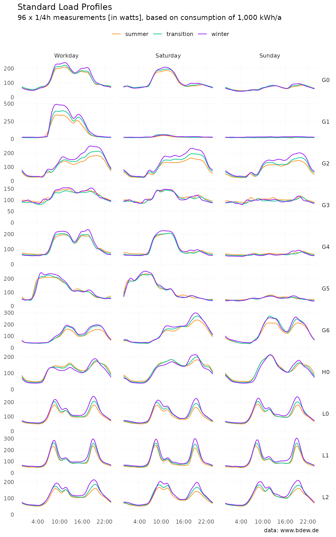
The data analysis revealed that load fluctuations for both commercial and agricultural customers remain moderate throughout the year. Specifically, for customers and customer groups labeled as G0 to G6, and L0 to L2,the standard load profile can be accurately derived directly from the 3x3 characteristic profile days available in the dataset slp.

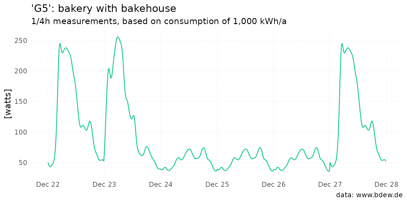
Below is the code snippet from the README, which can be used to reproduce the plot for the G5 profile, showcasing the algorithm’s outcome:

library(ggplot2)
ggplot(G5, aes(start_time, watts)) +
  geom_line(color = "#0CC792") +
  scale_x_datetime(
    date_breaks = "1 day",
    date_labels = "%b %d") +
  labs(
    title = "'G5': bakery with bakehouse",
    subtitle = "1/4h measurements, based on consumption of 1,000 kWh/a",
    caption = "data: www.bdew.de",
    x = NULL,
    y = "[watts]") +
  theme_minimal() +
  theme(
    panel.grid.minor.x = element_blank(),
    panel.grid.minor.y = element_blank(),
    panel.grid = element_line(
      linetype = "12",
      lineend = "round",
      colour = "#FAF6F4"
      )
  ) +
  NULL

As you can see, the values in 2023 for December 24 (a Sunday) and December 25 and 26 (both public holidays) are identical.

Special case: H0

In contrast to most commercial and agricultural businesses, which have a relatively even and constant electricity consumption throughout the year, household electricity consumption decreases from winter to summer and vice versa (at least in Germany). Because of the distinctive annual load profile characteristics of household customers, we contend that these customers cannot be adequately described through a static representation using 3x3 characteristic days, as is done for commercial or agricultural customers during the respective periods. Consequently, the values provided in the slp dataset are not directly comparable with the representative 1/4h values of commercial and agricultural profiles. In the context of the slp dataset, the term ‘static’ is somewhat inappropriate when applied to household profiles. The values for H0 within the slp dataset are primarily mathematical auxiliary values intended for multiplication with a dynamization factor.

This is taken into account when you call slp_generate(). The study suggested the application of a 4th order polynomial function to the values of standard load profile H0.

\[ w_d = w_s \times(-3.92\mathrm{e}{-10} \times d^4 + 3.20\mathrm{e}{-7} \times d^3 - 7.02\mathrm{e}{-5} \times d^2 + 2.10\mathrm{e}{-3} \times d + 1.24) \] Where:

• \(w_d\) is the resulting ‘dynamic’ value
• \(w_s\) is the ‘static’ value
• \(d\) is the day of the year as integer, starting at 1 on January 1st

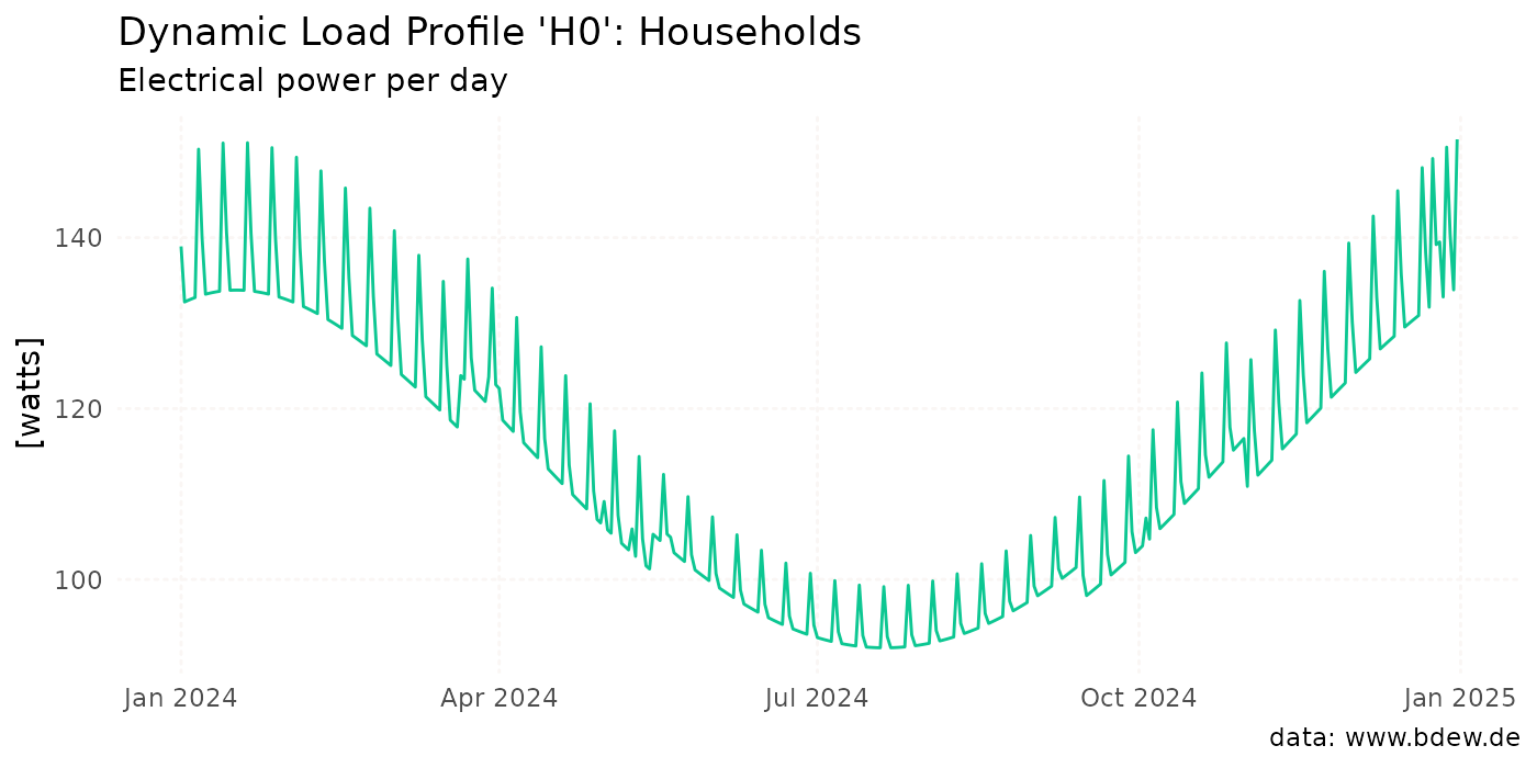
The following plot shows how the electrical power develops over the year for profile H0; for a clearer picture, the values are aggregated at daily level:

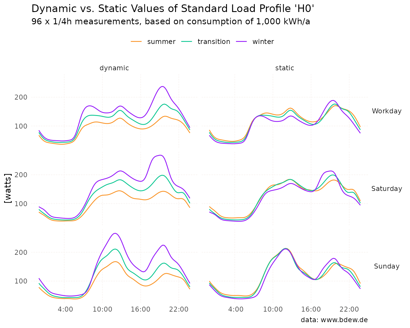
This multiplication process aims to generate a representative, dynamic load profile. Finally, the following chart compares the dynamic values with their static counterparts.⁴